1. Introduction

A PWM output can be easily transformed into an “analog” signal using low-pass filtering. This is the reason why Arduino calls its PWM output as analog. Nevertheless, the STM32F072 device features a real Digital to Analog Converter (DAC). When using DAC, you get closer to a real analog output as we will see in this tutorial.

2. DAC setup

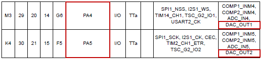
According to the device datasheet, there are two pins that can be used as DAC output: PA4 and PA5. As PA5 is already used by the board LED, we will only consider DAC Channel 1, attached to PA4.

For a basic functionality, the DAC setup is very simple. You just need to setup PA4 pin as analog, then turn on DAC clock and enable DAC. That’s all. Add the following function to your bsp.rs:

/*
 * bsp_dac_init()
 * Initialize DAC for a single output
 * on channel 1 -> pin PA4
 */

pub fn bsp_dac_init(peripherals: &Peripherals) {
    let (rcc, gpioa, dac) = (&peripherals.RCC, &peripherals.GPIOA, &peripherals.DAC);

    // Enable GPIOA clock
    rcc.ahbenr.modify(|_, w| w.iopaen().enabled());

    // Configure pin PA4 as analog
    gpioa.moder.modify(|_, w| w.moder4().analog());

    // Enable DAC clock
    rcc.apb1enr.modify(|_, w| w.dacen().enabled());

    // Reset DAC configuration
    dac.cr.reset();

    // Enable DAC Channel 1
    dac.cr.modify(|_, w| w.en1().enabled());
}

3. Sampling period setup

We want to output an analog sample from the DAC at regular time interval. Because we are unsure of the time it takes to compute sample, we will use a timer update event to trigger new samples on a regular basis. Adjust the previously developed TIM6 time base function so that update event (detected by polling UIF flag) occurs every 400µs:

/*
 * bsp_timer_timebase_init()
 * TIM6 at 48MHz
 * Prescaler   = 48 -> Counting period = 1µs
 * Auto-reload = 400  -> Update period   = 400µs
 */
pub fn bsp_timer_timebase_init(peripherals: &Peripherals) {
    let (rcc, tim6) = (&peripherals.RCC, &peripherals.TIM6);

    // Enable TIM6 clock
    rcc.apb1enr.modify(|_, w| w.tim6en().enabled());

    // Reset TIM6 configuration
    tim6.cr1.reset();
    tim6.cr2.reset();

    // Set TIM6 prescaler
    // Fck = 48MHz -> /48 = 1MHz counting frequency
    tim6.psc.modify(|_, w| w.psc().bits((48 - 1) as u16));

    // Set TIM6 auto-reload register for 400µs period
    tim6.arr.modify(|_, w| w.arr().bits((400 - 1) as u16));

    // Enable auto-reload preload
    tim6.cr1.modify(|_, w| w.arpe().enabled());

    // Start TIM6 counter
    tim6.cr1.modify(|_, w| w.cen().enabled());
}

4. Sinewave output

Add the following dependency in the "dependencies" section of your Cargo.toml:

libm = "0.2.2"

This added crate is a port of a C library called MUSL, which implements lightweight math functions like sin, cos, and many others.

In the example bellow, the DAC is used to output a sinewave.

...
extern crate libm;
use libm::sinf;
...

#[entry]
fn main() -> ! {
    // Variables
    let (mut angle, mut y): (f32, f32) = (0.0, 0.0);
    let mut output: u16;

    // Get peripherals
    let peripherals = Peripherals::take().unwrap();
    let (dac, tim6) = (&peripherals.DAC, &peripherals.TIM6);

    // Configure System Clock
    let _fclk = system_clock_config(&peripherals).unwrap();

    // Initialize LED pin
    bsp::bsp_led_init(&peripherals);

    // Initialize DAC output
    bsp::bsp_dac_init(&peripherals);

    // Initialize timer for delays
    bsp::bsp_timer_timebase_init(&peripherals);

    // Main loop
    loop {
        // Start measure
        bsp::bsp_led_on(&peripherals);

        // Increment angle value modulo 2*PI
        angle += 0.01;
        if angle > 6.28 {
            angle = 0.0
        }

        // Compute sinus(angle)
        y = sinf(angle);

        // Offset and Scale output to DAC unsigned 12-bit
        output = (0x07FFi16 + (0x07FF as f32 * y) as i16) as u16;

        // End measure
        bsp::bsp_led_off(&peripherals);

        // Set DAC output
        dac.dhr12r1.modify(|_, w| w.dacc1dhr().bits(output));

        // Wait for update event (one sample every 400µs)
        while tim6.sr.read().uif().is_clear() {}
        tim6.sr.modify(|_, w| w.uif().clear());
    }
}

The samples are calculated on-the-fly using the sinf function from libm library. sinf is faster than sin because it is written using simple precision floats instead of double precision floats.

The angle variable goes from 0 to 6.28 (2π, for those who wonder) by steps of 0.01 providing us with 628 samples for one period. Given that we have a 200µs period between samples, the sinewave period is:

$$f=\frac{1}{628\times400µs}=3.84585Hz$$

The sinf function returns a float number y in the range [-1 : 1]. The DAC data register is an unsigned 12-bit number [0 : 4095] that represents voltage between 0 and 3.3V. Therefore, for a full-scale 3.3Vpp sinewave, we have:

$$DAC_{output}=2047+(y\times2047)$$

Last thing, note that LED on PA5 is used to measure the time it takes to the CPU to compute and output the next sinus sample. We can use this to make sure that processing time is below the 200µs sampling period. If not, we have a problem...

Everything should be clear now. Save the code (Ctrl + S) and start a debug session.

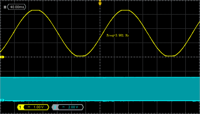
Probe PA4 and PA5 with an oscilloscope, and you should see this. The sinewave frequency and amplitude are in perfect agreement with the anticipated values.

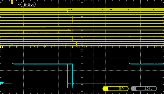
The application uses the LED pin to provide a measure of time required to compute a new sample. This method to measure execution time is simple and precise. You must use it whenever you need. Probing PA5 (channel 2 of the oscilloscope) reveals that the math part of the code requires between 173µs to 184µs to complete depending on the value of angle. The time the sinf function takes to deliver result is therefore not deterministic and depends on its operand. This is something usual you need to know.

The application will execute as expected as long as the sampling period accommodates the longest sample processing time. Here, 400µs are well enough to cope with sample calculation. Otherwise, the uniformity of the sampling is lost.

If you want to try the standard sin function, you will notice that it takes a longer time to complete (between 200µs to 300µs).

This is quite a long time, and the reason why math functions should be used with care when timing constraints are tight. Otherwise, you can use a Look-Up table (more on that later), or if you are rich, buy you a better CPU with hardware floating point unit (FPU). Cortex-M4 CPUs have one…

5. Summary

This short tutorial introduced the DAC peripheral and uniform sampling of digitized signals. It is a groundwork for further signal processing applications.