5.1. Digital filtering

1. Introduction

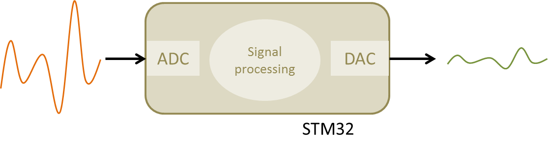
The purpose of this tutorial is to drive you though the design of a digital filter that takes an analog input signal applied to the ADC, then processes incoming samples, and finally provides an analog output using a DAC.

In the first part, the tutorial provides some basic background on digital filters. You may need some prerequisite knowledge, mostly on Laplace transform and z-transform, to get a full understanding of exposed matter, but you can still grab some useful tricks even if you are new to the field of digital filtering.

2. First order digital filter

2.1. The z-domain transfer function

The common representation of first-order Low-Pass filter transfer function in the Laplace domain is:

$$H(p)=\frac{1}{1+\tau p}$$

The cutoff frequency of such filter is given by:

$$\omega_c =\frac{1}{\tau}= 2\pi f_c$$

Let us suppose that we want a cutoff frequency $f_c=2Hz$. We therefore have:

$$\tau =\frac{1}{2\pi f_c}\approx 0.08$$

$$H(p)=\frac{1}{1+0.08\, p}$$

The Laplace variable p (or s if you live anywhere in the world but in France :-)) is useful to represent transfer functions in the continuous-time domain. When dealing with digital systems, incoming signal is sampled at regular time intervals. The Laplace transform is no more representative of such a discrete-time system.

The Laplace-transform equivalent for sampled signals is called the z-transform.

A common approach to move a Laplace transfer function into the z-domain is to use something called the “bilinear transform”. The bilinear transform is obtained by mapping z-plane to p-plane using:

$$z=e^{\, pT}$$

where T is the sampling period (in seconds). In the tutorial, we will use a 10ms sampling period (i.e. we will get a new input from ADC every 10ms).

The inverse mapping gives:

$$p=\frac{1}{T}ln(z)$$

Using first term of ln series expansion, we have:

$$p\approx \frac{2}{T}\frac{(z-1)}{(z+1)}$$

Applying the bilinear transform to our first order Low-Pass filter then gives:

$$H(p)=\frac{1}{1+\tau p}$$

$$H(z)=\frac{1}{1+\tau(\frac{2}{T}\frac{(z-1)}{(z+1)})}$$

$$H(z)=\frac{1}{\frac{T(z+1)+2\tau(z-1)}{T(z+1)}}$$

$$H(z)=\frac{Tz+T}{(T-2\tau)+z(T+2\tau))}$$

$$H(z)=\frac{\frac{T}{(T+2\tau)}+\frac{T}{(T+2\tau)}z}{\frac{(T-2\tau)}{(T+2\tau)}+z}=\frac{\alpha + \alpha z}{\beta+z}$$

With $T=0.01s$ and $\tau=0.08s$

$\alpha = \frac{T}{(T+2\tau)}=0.0588235$ and $\beta = \frac{(T-2\tau)}{(T+2\tau)}=-0.8823529$

The z-domain transfer function of our digital Low-Pass filter, sampled at 100Hz (T=10ms), and having a cutoff frequency of fc=2Hz is finally:

$$H(z) = \frac{0.0588235 + 0.0588235z}{-0.8823529+z}$$

 

2.2. On the use of Python as a z-domain transfer function calculator

Luckily for you, scientific computing software such as Matlab® or Scilab® are able to process linear systems transfer function from continuous-time to discrete-time (and reversely) quite easily. Here, I'll illustrate this by means of a Python script and the Scipy package.

The following script does the same bilinear transform as seen above:

from scipy import signal

# Build Laplace transfert function
s = signal.lti([1], [0.08, 1])

# Compute z-transform
sz = s.to_discrete(0.01, method='bilinear')

And the same with some plots:

from scipy import signal
import numpy as np
import matplotlib.pyplot as plt

# Build Laplace transfert function
s = signal.lti([1], [0.08, 1])

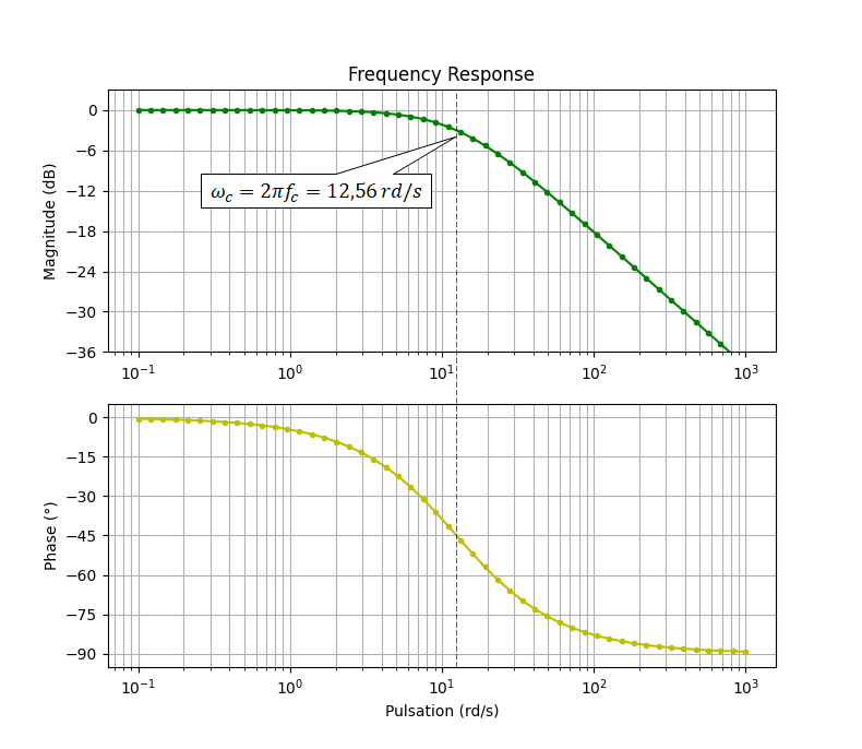
# Compute Bode plot
ws = np.logspace(-1, 3, 50)
w, mag, phase = s.bode(ws)

# Plot figure
fig = plt.figure(1)
fig.clf()

plt.subplot(211)
plt.title('Frequency Response')
plt.ylabel('Magnitude (dB)')
plt.semilogx(w,mag, 'g.-')
plt.ylim(-36, 3)
plt.yticks(np.arange(-36, 0 +1, step=6))
plt.grid(True,  which="both", ls="-")

plt.subplot(212)
plt.xlabel('Pulsation (rd/s)')
plt.ylabel('Phase (°)')
plt.semilogx(w,phase, 'y.-')
plt.ylim(-95, 5)
plt.yticks(np.arange(-90, 0 +1, step=15))
plt.grid(True,  which="both", ls="-")

plt.show()

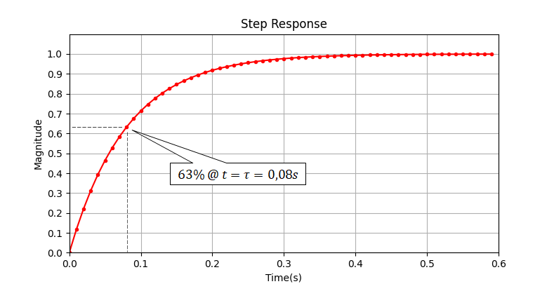
# Compute Step response
ts = np.arange(0, 0.6, step=0.01)
t, y = signal.step(s, T=ts)

# Plot figure
fig = plt.figure(2)
fig.clf()

plt.title('Step Response')
plt.xlabel('Time(s)')
plt.ylabel('Magnitude')
plt.plot(t,y, 'r.-')
plt.xlim(0, 0.6)
plt.ylim(0, 1.1)
plt.yticks(np.arange(0, 1.1, step=0.1))
plt.grid(True,  which="both", ls="-")

plt.show()

# Compute and z-transform
sz = s.to_discrete(0.01, method='bilinear')
print(sz)

 

Executing the above script provides the following outputs.

The obtained z-transfer function confirms the one we calculated earlier:

TransferFunctionDiscrete(
array([0.05882353, 0.05882353]),
array([ 1.        , -0.88235294]),
dt: 0.01
)

$$H(z) = \frac{0.05882353 + 0.05882353z}{-0.88235294+z}$$

 

2.3. From z-domain transfer function to software implementation

The z-transform is a discrete-time representation of the filter that relates output samples to input samples:

$$H(z) = \frac{\alpha + \alpha z}{\beta+z}=\frac{Y(z)}{X(z)}$$

Where $X(z)$ represents the input samples and $Y(z)$ represents the output samples.

Let us turn this into something more practical from a programming perspective:

$$\frac{Y(z)}{X(z)} = \frac{\alpha + \alpha z}{\beta+z}$$ $$Y(z)\beta + Y(z)z = X(z)\alpha + X(z)\alpha z$$

Above equation is processed each time a new sample is available. While X(z) represents the current incoming signal sample, X(z)z represents the sample that will come (in the future) the next sampling period. More generally, multiplying X(z) or Y(z) by $z^n$ is the same as putting an index n on the sample being processed.

• n = 0   → current sample
• n = 1   → next sample
• n = -1 → previous sample

Because no filter can predict what the future will be, we can divide all the parts of the above equation by z to have:

$$Y(z)\beta z^{-1} + Y(z) = X(z)\alpha z^{-1} + X(z)\alpha$$

$$Y(z) = X(z)\alpha z^{-1} + X(z)\alpha-Y(z)\beta z^{-1}$$

The $z^{-1}$ factor represents a delay of one sample. The above equation can therefore be written:

$$y_n = \alpha x_{n-1} + \alpha x_n -\beta y_{n-1}$$

$$y_n = \alpha(x_{n-1} + x_n) -\beta y_{n-1}$$

where:

•     $y_n$    is the output sample computed at the nth iteration
•     $y_{n-1}$ is the output sample computed at the (n-1)th iteration
•     $x_n$    is the input sample read at the nth iteration
•     $x_{n-1}$ is the input sample read at the (n-1)th iteration

The above equation is called the recursion equation, and can be directly applied to the filter computation within a program.

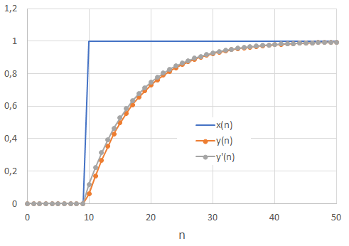
For instance, you can experiment the above equation with Excel (or any other tool you like):

•  Create a column of sample indexes n
•  Create a column of x input samples (some ‘0’ and then some ‘1’ for a step response)
•  Create a column for y outputs by using the above equation
•  Plot both x and y data with n as x-axis.

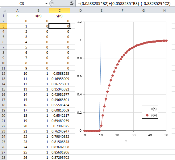
Looking at the above step response, you may recognize a first order low-pass filter. Moreover, you'll notice that time is not there since each output sample is calculated after both the previous one and the input sample. This should make clear in your mind that actual filter time constant $\tau$ now depends on the time interval between each sample calculation, i.e. the sampling period $T$ so that x-axis can be changed from $n$ the sample index into time $t$.

2.4. Further simplification

In the previous equation, we observe that each output sample calculation requires:

• One addition          → $x_{n-1} {\color{Red} \oplus} x_n$        
• Two products         → $\alpha {\color{Red} \otimes} (x_{n-1} + x_n)$ and $\beta {\color{Red} \otimes} y_{n-1}$
• Another addition    → $\alpha(x_{n-1}+x_n) {\color{Red} \oplus} -\beta y_{n-1}$

If we assume that the sampling frequency is high compared to input signal frequency (which is usually the case), we can further simplify our equation by assuming that $x_{n-1}$ and $x_{n}$ are not very different.

$$y_n=\alpha(x_{n-1}+x_n)-\beta y_{n-1}$$

with $x_{n-1}\approx x_n$

$$y_{n}^{'}\approx 2\alpha x_n-\beta y_{n-1}^{'}$$

Now, we can notice that:

$$2\alpha =\frac{2T}{(T+2\tau)}\; and\;  \beta=\frac{(T-2\tau)}{(T+2\tau)}$$

$$\beta+1=\frac{(T-2\tau)}{(T+2\tau)}+1=\frac{(T-2\tau)+(T+2\tau)}{(T+2\tau)}=\frac{2T}{(T+2\tau)}=2\alpha$$

$$2\alpha = \beta+1$$

The above equation rewrites:

$$y_{n}^{'}\approx (\beta+1) x_n-\beta y_{n-1}^{'}$$

Let us write

$$\gamma = (\beta+1)$$

$$y_{n}^{'}\approx \gamma x_n+(1-\gamma) y_{n-1}^{'}$$

With $\gamma = \frac{2T}{(T+2\tau)}$

We have removed one addition. Using again:

T=0.01s      τ=0.08s

We have finally:

$$y_{n}^{'}\approx 0.11765 x_n+0.88235 y_{n-1}^{'}$$

The plot below compares both step responses of first (y) and simplified (y’) version of our filter. Based on that result, we can accept the assumption that $x_{n-1}$≈$x_n$ and use the simplified form of the filter. We can also see that 63% of the final output value is reached at sample #18. That is 8 samples after the step is applied. With a sampling period of 0.01s, we confirm that τ=0.08. It now makes clear that the sampling period strongly determines the cutoff frequency of the filter. In other words, running the above equation at different sampling rate would provide different cutoff frequency.

Finally, note that the above approximation corresponds to the zero-order hold ('zoh') default method used within Scipy:

from scipy import signal

# Build Laplace transfert function
s = signal.lti([1], [0.08, 1])

# Compute z-transform
sz = s.to_discrete(0.01, method='zoh')

Giving a z-domain transfer function very close to the one obtained after simplification:

TransferFunctionDiscrete(
array([0.1175031]),
array([ 1.       , -0.8824969]),
dt: 0.01
)

$$H(z) = \frac{0.1175031}{-0.8824969+z}$$

 

3. Basic “analog follower” project

Before going into the filter implementation, let us prepare an application that simply copies the input voltage from the ADC channel to the DAC output. The next sections review the necessary setup for involved peripherals.

3.1. ADC configuration

Below is the setup for ADC. It is a one channel conversion therefore DMA is not involved:

/*
 * ADC_Init()
 * Initialize ADC for single channel conversion
 * - Channel 11 -> pin PC1
 */
void BSP_ADC_Init()
{
	// Enable GPIOC clock
	RCC->AHBENR |= RCC_AHBENR_GPIOCEN;

	// Configure pin PC1 as analog
	GPIOC->MODER &= ~(GPIO_MODER_MODER1_Msk);
	GPIOC->MODER |= (0x03 <<GPIO_MODER_MODER1_Pos);

	// Enable ADC clock
	RCC->APB2ENR |= RCC_APB2ENR_ADC1EN;

	// Reset ADC configuration
	ADC1->CR 	= 0x00000000;
	ADC1->CFGR1  = 0x00000000;
	ADC1->CFGR2  = 0x00000000;
	ADC1->CHSELR = 0x00000000;

	// Enable 12-bit continuous conversion mode
	ADC1->CFGR1 |= (0x00 <<ADC_CFGR1_RES_Pos) | ADC_CFGR1_CONT;

	// Select PCLK/2 as ADC clock
	ADC1->CFGR2 |= (0x01 <<ADC_CFGR2_CKMODE_Pos);

	// Set sampling time to 28.5 ADC clock cycles
	ADC1->SMPR = 0x03;

	// Select channel 11
	ADC1->CHSELR |= ADC_CHSELR_CHSEL11;

	// Enable ADC
	ADC1->CR |= ADC_CR_ADEN;

	// Start conversion
	ADC1->CR |= ADC_CR_ADSTART;
}

 

3.2. DAC configuration

Same thing for the DAC setup. We have a basic configuration:

/*
 * DAC_Init()
 * Initialize DAC for a single output
 * on channel 1 -> pin PA4
 */
void BSP_DAC_Init()
{
	// Enable GPIOA clock
	RCC->AHBENR |= RCC_AHBENR_GPIOAEN;

	// Configure pin PA4 as analog
	GPIOA->MODER &= ~GPIO_MODER_MODER4_Msk;
	GPIOA->MODER |= (0x03 <<GPIO_MODER_MODER4_Pos);

	// Enable DAC clock
	RCC->APB1ENR |= RCC_APB1ENR_DACEN;

	// Reset DAC configuration
	DAC->CR = 0x00000000;

	// Enable Channel 1
	DAC->CR |= DAC_CR_EN1;
}

 

3.3. Timebase configuration

TIM6 timebase is tuned for 10ms period between update interrupts:

/*
 * BSP_TIMER_Timebase_Init()
 * TIM6 at 48MHz
 * Prescaler   = 48000  -> Counting frequency is 1kHz
 * Auto-reload = 10 	-> Update period is 10ms
 * Enable Update Interrupt
 */
void BSP_TIMER_Timebase_Init()
{
	// Enable TIM6 clock
	RCC->APB1ENR |= RCC_APB1ENR_TIM6EN;

	// Reset TIM6 configuration
	TIM6->CR1 = 0x0000;
	TIM6->CR2 = 0x0000;

	// Set TIM6 prescaler
	// Fck = 48MHz -> /48000 = 1kHz counting frequency
	TIM6->PSC = (uint16_t) 48000 -1;

	// Set TIM6 auto-reload register for 10ms
	TIM6->ARR = (uint16_t) 10 -1;

	// Enable auto-reload preload
	TIM6->CR1 |= TIM_CR1_ARPE;

	// Enable Interrupt upon Update Event
	TIM6->DIER |= TIM_DIER_UIE;

	// Start TIM6 counter
	TIM6->CR1 |= TIM_CR1_CEN;
}

 

And NVIC is configure to allow TIM6 interrupts with priority 1:

/*
 * BSP_NVIC_Init()
 * Setup NVIC controller for desired interrupts
 */
void BSP_NVIC_Init()
{
	// Set priority level 1 for TIM6 interrupt
	NVIC_SetPriority(TIM6_DAC_IRQn, 1);

	// Enable TIM6 interrupts
	NVIC_EnableIRQ(TIM6_DAC_IRQn);
}

 

3.4. Follower stage

Finally, the main() function implementing follower stage is given below. in and out variables have been set as global in order to allow STM-Studio® monitoring:

// Global variables
...
uint8_t	timebase_irq = 0;
uint16_t	in, out;

// Main program
int main()
{
	// Configure System Clock
	SystemClock_Config();

	// Initialize 10ms timebase
	BSP_TIMER_Timebase_Init();
	BSP_NVIC_Init();

	// Initialize ADC
	BSP_ADC_Init();

	// Initialize DAC
	BSP_DAC_Init();

	// Initialize LED pin
	BSP_LED_Init();

	// Main loop
	while(1)
	{
		// Do every 10ms
		if (timebase_irq == 1)
		{
			// Start measure
			BSP_LED_On();

			// Input signal <-- ADC
			while ( (ADC1->ISR & ADC_ISR_EOC) != ADC_ISR_EOC );
			in = ADC1->DR;

			// Follower stage
			out = in;

			// Output signal --> DAC
			DAC->DHR12R1 = out;

			// Stop measure
			BSP_LED_Off();
			timebase_irq = 0;
		}
	}
}

 

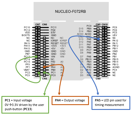
In order to test the follower stage, let us connect the user button pin PC13 to the ADC input pin PC1. This is a convenient way to generate full-scale input steps (0V → 3.3V) to the filter input pin PC1. Make sure that you have no code processing the push-button event. You don’t even need to call the BSP_PB_Init() function as all pins are input upon reset and we’re not going to read button state anyway.

Save all , build  and run  the application.

If you have an oscilloscope at hand, you can make some verifications:

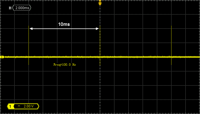
•     Probing PA5, you should see a short pulse that occurs every 10ms, according to the settings of the timebase:

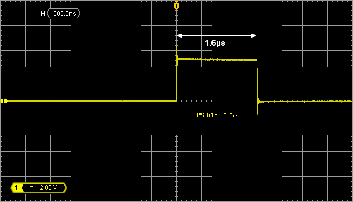
• Zooming horizontal, the width of the PA5 pulse tells you about the time it takes to execute the filter loop. At this moment, the process takes 1.5µs to complete. Remember that we are doing nothing more than output = input (follower stage). It has to be short…

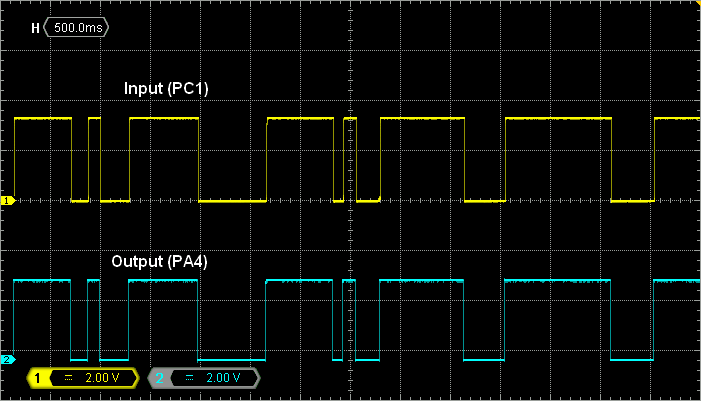
• Probing both PC1 and PA4 and playing with the user push-button, you can make sure that the follower stage actually follows (DAC output on PA4 is a copy of ADC input on PC1):

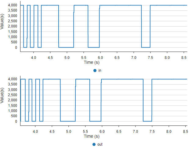
Alternatively, you can monitor both in and out variables with STM32CubeMonitor while playing with the user button:

When you have checked that everything is working as expected, you are ready to start the filter implementation.

Commit name "Digital filter - Follower"   Push onto Gitlab

 

4. Filter implementation

Remember that our filter is described by the following recursion equation:

$$y_{n}= 0.11765 x_n+0.88235 y_{n-1}$$

$$y_{n}= c_1\times x_n+c_2\times y_{n-1}$$

In a first time, we will implement this equation directly using floats for the two coefficients $c_1$ and $c_2$.

4.1. Floating point arithmetic

Edit the main() function as shown below.

...

int main()
{
	float c1, c2;	// Filter coefs
	float x = 0;	// Filter input
	float y = 0;	// FIlter output

	...

	// Setup filter coefs
	c1 = 0.11765f;
	c2 = 0.88235f;

	// Main loop
	while(1)
	{
		// Do every 10ms
		if (timebase_irq == 1)
		{
			// Start measure
			BSP_LED_On();

			// Input signal <-- ADC
			while ( (ADC1->ISR & ADC_ISR_EOC) != ADC_ISR_EOC );
			in = ADC1->DR;

			// Filter stage
			x = (float)in;
			y = (c1*x) + (c2*y);
			out = (uint16_t)y;

			// Output signal --> DAC
			DAC->DHR12R1 = out;

			// Stop measure
			BSP_LED_Off();
			timebase_irq = 0;
		}
	}
}

Note that in y = (c1*x) + (c2*y) we already have yn on the left-hand side of '=' and yn-1 on the right-hand side.

Build the project and run.

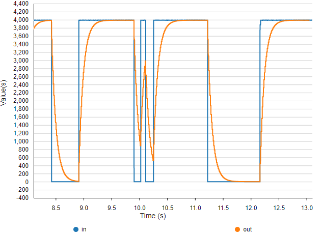
You can use STM32CubeMonitor to get a quick view on the result:

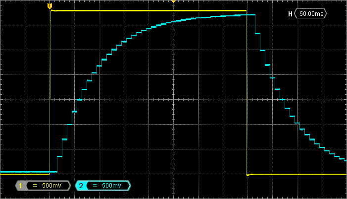
For precise measurements, it’s better using an oscilloscope. Probe both input (PC1) and output (PA4) pins:

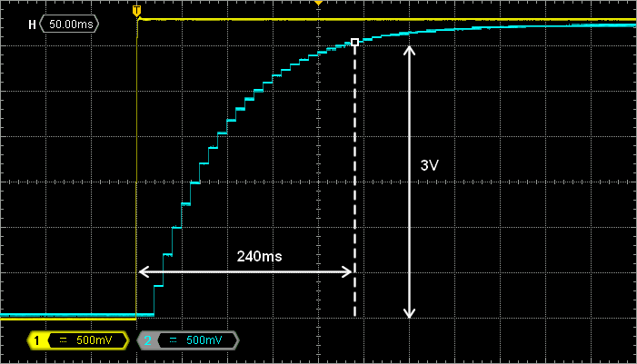
Remember that we want  τ =80ms. About 95% of the final value should be reached within 3τ = 240ms. The figure above is a detailed view of the step (push-button) response. We can see that the filter behaves perfectly as expected. The filter final value is almost reached after 5τ.

Next, probe PA5 (filter processing time).  In the figure below, we first note that the filter is processed quite fast compared to the sampling period (10ms), meaning that CPU is spending most of the time doing nothing, waiting for the next time base interrupt.

We can measure an execution time of about 16µs:

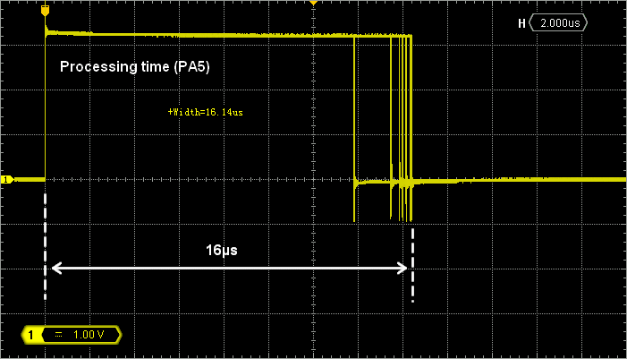
If you play with the user Push-Button, you may notice that the processing time is not the same when input signal is high or low. It is actually a little bit faster (13.4µs) when input is 0 (button down) because arithmetic operations are likely simplified with null operands. Therefore, one can see that computation time is not deterministic, and depends on operands values. That’s a consequence of conditional branches in the assembly code that result from floating point arithmetic synthesis.

Commit name "Digital Filter - Floating point arithmetics"   Push onto Gitlab

 

4.2. Fixed point arithmetic

Using float type to represent real numbers such as our coefficients c1 and c2 is a natural thing for you, but not for a CPU that can only perform maths on integers. Real numbers may also be represented by binary numbers, assuming a virtual decimal point somewhere in between bits. Such representation is called fixed-point representation (‘float’ being for floating-point representation).

We are aware that Cortex-M0 CPU does not have any dedicated hardware to perform floating point arithmetic (Floating Point Unit, FPU). So it is likely that using floats is slowing down code execution (i.e. floating point arithmetic produces many assembly lines to complete).

Try the code below where filter variables are represented by a 12-bit decimal place fixed-point:

...
// Main program
int main()
{
	uint16_t c1, c2;   // Filter coefs
	uint16_t x = 0;    // Filter input
	uint32_t y = 0;    // Filter output

	...

	// Setup filter coefs
	c1 = 482;	// 0.11765f *2^12
	c2 = 3614;	// 0.88235f *2^12

	// Main loop
	while(1)
	{
		// Do every 10ms
		if (timebase_irq == 1)
		{
			// Start measure
			BSP_LED_On();

			// Input signal <-- ADC
			while ( (ADC1->ISR & ADC_ISR_EOC) != ADC_ISR_EOC );
			in = ADC1->DR;

			// Filter stage
			x = in;
			y = (c1*x) + (c2*y);
			y = (y >>12U);		// Remove decimal part
			out = y;

			// Output signal --> DAC
			DAC->DHR12R1 = out;

			// Stop measure
			BSP_LED_Off();
			timebase_irq = 0;
		}
	}
}

Build the project and flash the target.

Make sure that the filter behaves exactly as before (i.e.  when using floats):

If you are using STM32CubeMonitor, you can also see the filter behavior:

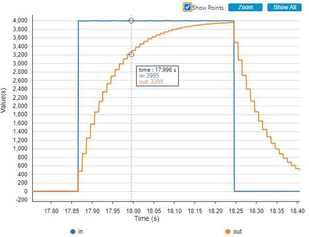
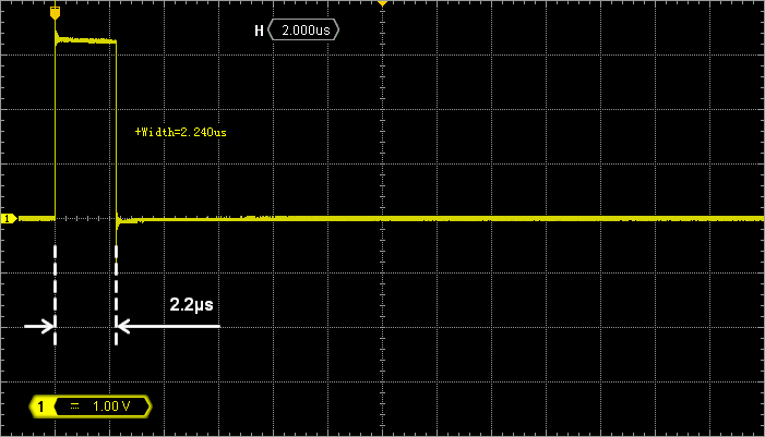
When this is done, use the PA5 pin to measure the filter processing time. You’ll find that this implementation is about 8x faster (2µs) than the one using floats. For the very same behavior! Play with the user button and you will also notice that processing time is now deterministic (i.e. computation time does not depend on operands). That's very good indeed.

 

Commit name "Digital filter - Fixed point arithmetics"   Push onto Gitlab

 

5. Summary

In this tutorial, you have implemented a digital low-pass filter. With a little help from Matlab®, Scilab® or Python, you should be able to synthesize in the digital domain any filter as long as you have its transfer function in the Laplace form.

The tutorial took you into 2 coding approaches, the second being 8x faster that the first one for the very same result.

Processing efficiency depends on your coding skills. It has consequences on application performance and more generally on the business (money).

A code that is more efficient allows you:

• to buy a less powerful, less expensive processor for the same task
• to reduce MCU clock speed and therefore reduce power consumption (i.e. increase battery life in the case of mobile application, reduce heat dissipation requirements…)
• spend more time in low-power modes

These benefits are not just “icing on the cake”. It is fundamental that you produce efficient code every time you can.